Outlier Detection using Generative Adversarial Networks

Abstract

Outlier detection techniques are widely used for solving tasks such as fraud detection, anomalous tissue detection in medical imaging data, or improving voice recognition models. By cleaning training datasets of outlying data points, unsupervised machine learning algorithms also benefit from a significant performance increase.

This report investigates the Generative Adversarial Network model, a technique for training generative models to learn the underlying probability distribution of an arbitrary training dataset through discriminative means. The work carried on in this project shows how the latent space of a Generative Adversarial Network model can be exploited for the task of outlier detection in Computer Vision tasks, as well as providing an extension that allows a Generative Adversarial Network to detect outliers in generic, high-dimensional datasets.

Acknowledgements

I want to thank my supervisor, Mahesan Niranjan, for the freedom and encouragement for pursuing a project of my choice.

To M.B.

Chapter 1 - Introduction

The adoption of deep learning models in various fields of study has increased in recent years due to the reduced cost of training, and state of the art performance. This boost in performance and accuracy of deep learning models can be attributed, in part, to the prevalence of large-scale datasets for various tasks and fields of study.

With datasets such as the ImageNet Large Scale Visual Recognition Challenge [1ImageNet Large Scale Visual Recognition ChallengeRussakovsky, O., Deng, J., Su, H., et al. · 2015International Journal of Computer Vision 115(3), pp. 211–252], which currently contains over 9 million images, the human effort required for sifting through these datasets for data cleaning and outlier removal purposes increases exponentially, to the point of intractability.

Besides playing a big part in improving the accuracy and performance of machine learning models, outlier detection algorithms have deep practical ramifications in today’s data-driven world. Currently, outlier detection mechanisms are being used for a range of activities, including, but not limited to building robust voice recognition models and fraudulent activity detection.

The Generative Adversarial Network (GAN) model is a breakthrough method for training neural networks to imitate arbitrary data distributions, which consistently outperforms strictly generative models in high-dimensional tasks such as image generation [2Generative Adversarial NetsGoodfellow, I., Pouget-Abadie, J., Mirza, M., Xu, B., Warde-Farley, D., Ozair, S., Courville, A., Bengio, Y. · 2014Advances in Neural Information Processing Systems 27, pp. 2672–2680].

Given such performance of the GAN model, we hypothesise that a GAN-based outlier detection system will be able to outperform strictly generative models for outlier detection.

In this project, we leverage the power of GANs to learn and imitate specific data distributions in order to build a GAN-based algorithm for outlier detection in high-dimensional datasets.

Chapter 2 - Background Literature

2.1 Current state of Outlier Detection algorithms

The task of outlier detection, also referred to as anomaly or novelty detection, involves training an algorithm to identify test data which is significantly different to the training data. Outlier detection algorithms borrow techniques from various fields of study, including statistics and immunology.

Most of these algorithms aim to learn to model ’normality’, and then identify outliers using various metrics of dissimilarity between their learned model of ’normality’ and the test data.

According to Pimentel et al. [3A Review of Novelty DetectionPimentel, M. A. F., Clifton, D. A., Clifton, L., Tarassenko, L. · 2014Signal Processing 99, pp. 215–249], outlier detection systems follow five general categories: probabilistic, distance-based, reconstruction-based, domain-based and information-theoretic techniques.

2.1.1 Probabilistic methods

Probabilistic outlier detection systems use a generative model to learn the probability density of normality. Their assumption is that test data that lies in regions of low probability density has a higher likelihood of being anomalous. Most of these probabilistic models impose a threshold on the likelihood of a test candidate belonging to the ’normal’ class, and flag all data that falls under this imposed threshold.

Probabilistic methods can be split into parametric and non-parametric models.

Parametric models, like the Gaussian Mixture Model (GMM), make assumptions about the distribution of the data. In GMMs, this extends to assuming that the data distribution can be estimated from a weighted sum of Gaussian distributions, parameterised by the number of Gaussian prototypes considered.

Non-parametric models, such as Kernel Density Estimation (KDE), do not assume a fixed structure to a model. In the case of KDE, the functional form of the data distribution is estimated from the individual contributions of kernels placed on each data point in the dataset. In most cases, these kernels are Gaussian distributions.

While these models are simple to implement, and their outputs can be investigated using standard statistical tools, probabilistic models suffer from performance degradation when applied to high-dimensional datasets. The increase in dimensionality also increases the volume occupied by the data in the higher dimensional space, and thus sparsity. Sparse datasets can cause the estimated distribution to be wildly different to the actual distribution of the data.

2.1.2 Distance-based methods

Distance-based methods usually employ the use of clustering or nearest-neighbour methods for outlier detection. Their premise is that anomalous data will have an increased distance to its nearest neighbours, compared to normal data.

Even though these methods do not require us to impose prior assumptions on the training data, algorithms such as k-nearest neighbours do require suitable distance measures between data points. Inspecting high-dimensional datasets using distance-based methods is computationally expensive, as we need to compute the distance from each point to every other point in the dataset in order to determine the nearest neighbours. These methods can also suffer from the sparsity brought by increasing dimensionality.

2.1.3 Reconstruction-based methods

In reconstruction-based algorithms, a model of normality is learned by performing regression on the clean dataset. A reconstruction error is then computed between the regression target and the value of the test candidate when mapped using the regression model. Since outliers were not accounted for during training, these will have a larger reconstruction error than clean data, and thus they can be flagged for removal.

Some of the reconstruction-based methods include neural network models such as Multilayer Perceptrons or Autoencoders. In Autoencoder-based solutions, the model is trained to learn to replicate the input through an arbitrary number of hidden layers. Outliers are then detected when attempting to reconstruct a test candidate leads to a high reconstruction loss.

Pimentel et al. [3A Review of Novelty DetectionPimentel, M. A. F., Clifton, D. A., Clifton, L., Tarassenko, L. · 2014Signal Processing 99, pp. 215–249] describe these methods, and especially neural-network-based approaches, as sensitive to changes in hyperparameters, especially when using high-dimensional datasets.

2.1.4 Domain-based methods

Domain-based methods attempt to enclose the ’normal’ data inside a boundary. This is similar to the probabilistic methods, yet these models are insensitive to the density of the data. Here, outliers are identified based on their location, and whether they are a member of the domain of the training data.

Because this membership problem is very similar to a two-class classification problem, Support Vector Machines (SVMs) are a very popular technique for domain-based outlier detection.

2.1.5 Information-theoretic models

With information-theoretic models, we use techniques such as entropy to compute the information in a dataset.

These models assume that anomalies will significantly alter the entropy of a ‘clean’ dataset. Therefore, by computing the information content of the whole dataset, including outliers, and then progressively removing subsets from the dataset, we can identify subsets containing outliers from the large information loss suffered in response to removal.

However, depending on the metric used, these models may only be reliable when a big number of anomalous entries are present in the dataset.

2.2 The Generative Adversarial Network Model

At its core, a neural network uses matrix multiplications parameterised by weights in order to compute linear transformations of the input. In order to train a network to learn a task, the weights of the matrix multiplications have to be updated to bring our network’s output as close as possible to the desired target. This is achieved by computing an objective loss function between the output and the target, and then performing backpropagation to update the weights with respect to the loss value.

By optimising the model so that its predictions are as close to their respective target labels as possible, the model can achieve good prediction results during tests on unseen data.

A model can also be trained in an unsupervised manner, by not providing labels against which our model’s predictions are compared. This can allow the model to learn its own representations for the training data, potentially leading to more complex feature extraction, and pattern identification that was not obvious to a human observer. All of these can help increase the performance of the model and provide more meaning for a human investigating the dataset.

The Generative Adversarial Model is a neural network model that is trained using a semi-supervised approach. Here, the neural network model does not aim to optimise a single objective loss function, but instead it aims to achieve an equilibrium between two adversaries, where neither of them can make a gain from a strategy change, provided the adversary’s strategy remains constant.

In GANs, these two adversaries are the generator and the discriminator. The discriminator’s aim is to distinguish between samples that came from the training data distribution and samples that came from the generator’s distribution. The only set of labels provided to the discriminator are the origin of the data it has just seen, namely, whether it came from the training set, or it was generated by the generator. On the other hand, the generator’s aim is to create realistic samples that are ambiguous to the discriminator, causing it to misclassify generated data coming from the generator as training data.

This adversarial game played by the generator and discriminator can be described using the minimax decision strategy found in Game Theory, as the generator attempts to minimise the maximum loss that it can incur from the discriminator’s decision.

2.2.1 Structure

In a GAN, the two adversaries engaged in a minimax game are represented by neural networks. The discriminator’s goal is to maximise the accuracy with which it can distinguish real samples that came from the training set from fake samples that were generated by the generator. At the same time, the generator is trying to minimise the likelihood that its generated samples are identified as being fake by the discriminator.

As the discriminator learns to better model and extract patterns for discerning between training and fake data, the only way for the generator to ‘keep up’ with the discriminator’s progress is for it to progressively mimic the training data distribution with increasing accuracy.

At the end of the adversarial training, the generator’s samples are so accurate that the discriminator is unable to distinguish training (real) data from generated (fake) data.

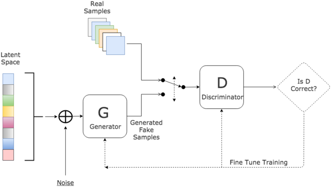
The adversarial game played by the generator and discriminator can be explained through the analogy of the bank and the currency forger. Here, the generator plays the role of a currency forger trying to produce counterfeit currency. The bank, played by the discriminator, will investigate the notes produced by the forger and give a response on whether or not the currency is real or counterfeit. In the case where the notes are declined by the bank for being counterfeit, the forger will alter the counterfeiting process, thus producing a different counterfeit note. The bank also alters its checking process to account for this new counterfeiting method. This process is repeated until the bank is unable to tell fake notes apart from real notes. In this case, the rate at which the bank erroneously rejects legitimate notes is the same as the rate at which the bank erroneously accepts counterfeit notes.

2.2.2 Training Algorithm

As stated above, a Generative Adversarial Network (GAN) is comprised of two neural network adversaries: the generator $G$, and the discriminator $D$.

The generator aims to generate output that could be realistically mistaken for samples taken from the training set, $\mathbf{X} = \{X^{(1)}, X^{(2)}, \ldots, X^{(n)}\}$. Thus, we aim to train the generator to learn a mapping $G(z; \theta_G)$, so that when given a random vector $z$ as input, the generator’s outputs will follow a probability distribution $p_G$ that is similar to the probability distribution of the training data, $p_X$.

During training, the parameters of the generator, $\theta_G$, are optimised to improve the output of $G$.

The random input vector $z \sim p_z$ is sampled from an arbitrary probability distribution $p_z$, which is typically either a uniform or a normal distribution. The probability distribution $p_z$ constitutes the latent space of the generator.

The discriminator $D(X^{(i)}; \theta_D)$, where $\theta_D$ models the parameters of the discriminator network and $X^{(i)}$ represents a feature vector sampled from the training set $\mathbf{X}$, is trained to output the probability that a certain data point $X^{(i)}$ came from the training data rather than from $p_G$ [2Generative Adversarial NetsGoodfellow, I., Pouget-Abadie, J., Mirza, M., Xu, B., Warde-Farley, D., Ozair, S., Courville, A., Bengio, Y. · 2014Advances in Neural Information Processing Systems 27, pp. 2672–2680].

The two networks D and G are played against each other in a two-player minimax game where the generator tries to ‘fool’ the discriminator that the generated data actually came from the training set. This game can be represented mathematically as $V(D, G)$ [2Generative Adversarial NetsGoodfellow, I., Pouget-Abadie, J., Mirza, M., Xu, B., Warde-Farley, D., Ozair, S., Courville, A., Bengio, Y. · 2014Advances in Neural Information Processing Systems 27, pp. 2672–2680]:

After training, the discriminator’s prediction accuracy should be no better than chance, i.e. 50%, as the generator’s samples are almost identical to the training data. At this stage, sampling data from $p_X$ or $p_G$ is synonymous.

Algorithmically, the process of training a Generative Adversarial Network can be represented as in Algorithm 1.

Algorithm 1 — GAN training.

G(z; θ_g) ← build generator
D(X; θ_d) ← build discriminator
for epoch ∈ [0, number of epochs):
    z          ← sample noise {z⁽¹⁾, z⁽²⁾, …, z⁽ᵐ⁾} from p_z
    data_real  ← sample data  {X⁽¹⁾, X⁽²⁾, …, X⁽ᵐ⁾} from p_X
    data_fake  ← G(z; θ_g)
    loss_D_real ← E_{x∼p_X(x)}  [log D(data_real; θ_d)]        // cross entropy
    loss_D_fake ← E_{z∼p_z(z)}  [log(1 − D(G(z; θ_g); θ_d))]   // cross entropy
    loss_D      ← loss_D_real + loss_D_fake
    θ_d        ← backpropagate(loss_D)
    z          ← sample noise {z⁽¹⁾, z⁽²⁾, …, z⁽ᵐ⁾} from p_z
    loss_G      ← E_{z∼p_z(z)}  [log D(G(z; θ_g); θ_d)]        // cross entropy
    θ_g        ← backpropagate(loss_G)

2.2.3 Implementing GAN architectures

In the original paper by Goodfellow et al. [2Generative Adversarial NetsGoodfellow, I., Pouget-Abadie, J., Mirza, M., Xu, B., Warde-Farley, D., Ozair, S., Courville, A., Bengio, Y. · 2014Advances in Neural Information Processing Systems 27, pp. 2672–2680], the generator is a multilayer perceptron with its input being a single noise vector z and output having the same dimensions as the training data.

The discriminator is also represented as a multilayer perceptron, taking in a feature vector with the same shape as the shape of the training data, and outputting a single scalar value between 0 and 1.

The output shape of the generator must match the input shape accepted by the discriminator, as the generator’s output is being fed directly into the discriminator.

After setting up the two neural networks, the next step is to define the loss function for the discriminator and the generator.

The output of the discriminator is bounded between 0 and 1, with 0 meaning that the input is predicted to have come from the training set and 1 meaning that the input has been generated by the generator.

In order to compute the loss, the output of the discriminator is compared against the labels (0 and 1) using the sigmoid cross-entropy function $S(H(p, q))$. This function is bounded in the range [0; 1], and therefore its output will constitute the probability of a sample being fake.

The sigmoid cross-entropy function is the function composition of the cross-entropy function and the sigmoid function $S(H(p, q))$, where $p$ and $q$ are probability distributions, and $H(p, q)$ and $S(x)$ are defined in Equation 2 and Equation 3 respectively.

The generator’s loss is derived by computing the sigmoid cross-entropy between a zero vector and the discriminator’s output when given the generator’s output as input.

By setting up the model’s losses in this way, the Network behaves in accordance to the adversarial minimax game defined in Equation 1.

To compute the gradients and update each model’s weights, the original paper suggests using stochastic gradient descent. However, faster convergence, as well as prevention of converging to a local optimum, can be achieved by substituting stochastic gradient descent for the Adam optimiser [5Adam: A Method for Stochastic OptimizationKingma, D. P., Ba, J. L. · 2015ICLR].

2.2.3.1 Best practices

Optimising a GAN can be thought of as reaching a Nash equilibrium between the generator and the discriminator, where none of the two can make a gain based on a unilateral change in strategy, given that the other adversary’s strategy remains constant.

This method of optimisation, despite its intuitive nature, makes it very difficult to train GANs to convergence, and makes the training process very unstable and noisy.

While efforts have been made to stabilise GAN training, through the invention of the Wasserstein GAN [6Wasserstein GANArjovsky, M., Chintala, S., Bottou, L. · 2017ICML], training GANs is still an ambiguous process that many times feels like interacting with a black box.

This section was written to demystify and troubleshoot common problems that arise during GAN training. By reading this section, the reader can understand some of the best practices that should be employed when training GANs.

One of the first difficulties encountered when training GANs is the possibility of having vanishing gradients for the generator.

In the vanishing gradient problem, the gradients computed when calculating the loss are so small that the changes backpropagated through the network are insignificant. This leads to the network converging to a sub-optimal solution.

One way of solving this problem is to simply switch over the ‘fake’ / ‘real’ labels, so that 0 now represents ‘fake’ and 1 represents ‘real’. An alternative would be to change the optimisation of the generator, so that instead of minimising $\log(1 - D(G(z)))$, the generator could be maximising $\log D(G(z))$.

Secondly, sampling the random noise vector z from a normal distribution yields much better results than sampling from a uniform distribution. This discovery was made when I noticed a performance improvement in the experiments detailed in Chapter 3 following this change.

Thirdly, a big performance increase can be brought to the model by scaling the input to the discriminator to have zero mean and unit variance. This can be done in the generator by using the hyperbolic tangent function, tanh as the output of the final layer of the generator, thus making the generated data only have values between -1 and 1.

Moreover, maintaining zero mean and unit variance throughout the network, as the input passes from one layer to another is a good way of preventing the vanishing gradient problem. This can be done by implementing batch normalisation between the layers of the network.

Another big performance increase comes from preventing the network from overfitting. Overfitting in GANs happens when the generator only learns to imitate a certain part of the distribution of the discriminator, yet the discriminator can still be fooled to think that the data resembles the training data. To avoid this, a good practice is using dropout, a technique that turns off random neurons in the network at a certain rate, thus forcing the model to find new pathways for arriving at the correct output. This technique should be implemented in both the generator and the discriminator. Experimentally, I found that a rate of 0.5 is enough to prevent overfitting.

Finally, mode collapse is a big issue that arises when attempting to train GANs to learn multimodal distributions.

In this case, a generator can learn to only generate realistic samples from one of the peaks of the distribution, thus still bypassing the discriminator’s checks, without learning the full distribution of the training data. This is problematic, as the discriminator will eventually catch up, learning to discredit samples coming from that certain peak.

In this case, there is a chance that the generator will ‘jump’ to generating samples from the other peak of the multimodal distribution, leading to a process that will continue ad nauseam , with neither the generator nor discriminator converging to an optimal solution

In the case of mode collapse, one solution involves evaluating an entire sample of generated data, rather than individual samples, thus encouraging diversity. Another technique involves showing fake samples from previous training epochs to the discriminator, to prevent it from ‘forgetting’ the previous techniques employed by the generator.

Chapter 3 - Framework implementation

3.1 Experimentation with GAN

Early experiments revolved around renowned GAN papers such as Radford et al. [7Unsupervised Representation Learning with Deep Convolutional Generative Adversarial NetworksRadford, A., Metz, L., Chintala, S. · 2015ICLRDCGAN.] and Goodfellow et al. [2Generative Adversarial NetsGoodfellow, I., Pouget-Abadie, J., Mirza, M., Xu, B., Warde-Farley, D., Ozair, S., Courville, A., Bengio, Y. · 2014Advances in Neural Information Processing Systems 27, pp. 2672–2680], and involved reimplementing the authors’ models and replicating their results.

The purpose of the work conducted in this chapter was to understand the GAN model and proper training of GANs, so that I could be well equipped to tackle building an outlier detection model using GAN.

3.1.1 Imitating a 1D Gaussian distribution

We constructed a GAN based on Goodfellow et al. [2Generative Adversarial NetsGoodfellow, I., Pouget-Abadie, J., Mirza, M., Xu, B., Warde-Farley, D., Ozair, S., Courville, A., Bengio, Y. · 2014Advances in Neural Information Processing Systems 27, pp. 2672–2680], using two adversarial multilayer perceptrons as the discriminator-generator adversarial pair.

The training data input to the discriminator consisted of batches of 100-dimensional vectors sampled from a one-dimensional normal distribution with mean $\mu = 4$ and standard deviation $\sigma = 1.25$. The input to the generator consisted of batches of 100-dimensional vectors sampled from a uniform distribution between -1 and 1.

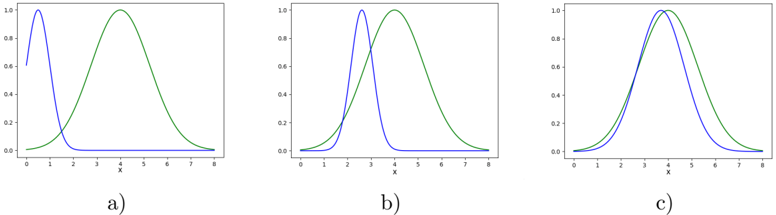
For this experiment, the GAN has been trained for 20000 epochs using a modification of mini-batch gradient descent, the Adam optimiser [5Adam: A Method for Stochastic OptimizationKingma, D. P., Ba, J. L. · 2015ICLR].

Following the authors’ hyperparameter configuration, and using two multilayer perceptrons as the generator and discriminator, I arrived at the same results as the authors, which can be seen in Figure 2.

3.1.2 Imitating a high dimensional wine property dataset

Even though Section 3.1.1 is a clear indication that GANs are capable of imitating and generating vectors that have a normal distribution of arbitrary mean and variance, this can be considered an easy task, as it only involves learning a mapping from one 100-dimensional space to another 100-dimensional space.

Therefore, I investigated whether GANs are capable of imitating distributions that were not artificially generated, such as our normal distribution in Section 3.1.1.

For this, I chose to see whether a GAN can learn the underlying probability distribution of an 11-dimensional dataset representing sets of chemical properties of various wines from the Wine Quality dataset by Cortez et al. [8Modeling Wine Preferences by Data Mining from Physicochemical PropertiesCortez, P., Cerdeira, A., Almeida, F., Matos, T., Reis, J. · 2009Decision Support Systems 47(4), pp. 547–553].

This dataset is made up of 6497 12-dimensional feature vectors representing various properties of red and white wines, including their alcohol by volume content, pH and residual sugar. The last component of the vectors represents the wine quality. I stripped away this component, considering it as a label to be used for regression/classification tasks.

Table 1. First four entries from the wine quality dataset. Some columns were omitted for visibility; a full description of the dataset is available in Appendix D.

Part of the first four entries of the dataset is shown in Table 1 (some columns were excluded for visibility).

This dataset constitutes a good choice for a GAN benchmarking experiment, as it is a high dimensional dataset, with feature vectors spanning 11 dimensions. Another property of this dataset is that it is not normally distributed, thus posing more of a challenge for a GAN imitating this distribution.

The only change to the model that was needed when moving from the 1-dimensional case presented in Section 3.1.1, was increasing the width of the input, output and hidden layers of both the generator and the discriminator, in order to allow the GAN to have more expressive power.

The hyperparameter configuration of this model can be found in Appendix A.

As suggested in Section 2.2.3.1, the dataset was scaled so that each feature has zero mean and unit variance. This is generally a good practice in any situation when training GANs, as it prevents issues such as vanishing/exploding gradients during backpropagation. In this case, this choice serves to reduce the sparsity in the dataset, and help the generator learn the data distribution easier.

Without scaling, different features of the dataset differ, in some cases, by orders of magnitude. For example, the value of sulfur dioxide in a wine could be as high as 440, while the volatile acidity could be as low as 0.08.

This could prove problematic, as it forces the generator to learn a very sparse distribution, and it means that the weights have to be optimised in such way that the generator is able to generate both very large numbers, as well as subunitary values.

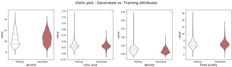
Training the GAN for 30,000 epochs using the Adam optimiser [5Adam: A Method for Stochastic OptimizationKingma, D. P., Ba, J. L. · 2015ICLR], the generator successfully learns how to generate wines with realistic properties that follow the properties of the training dataset. This is clearly seen in the violin plot in Figure 3, where the generator captures the mean and spread of each feature. Tables 2 and 3 also show samples from the generator and the training data to emphasise this.

Table 2. Wine samples from the training data distribution.

Table 3. Wine samples from the generator’s distribution. Each feature vector was scaled back to the original size.

Note: the data presented above was rescaled back to the original values before presentation.

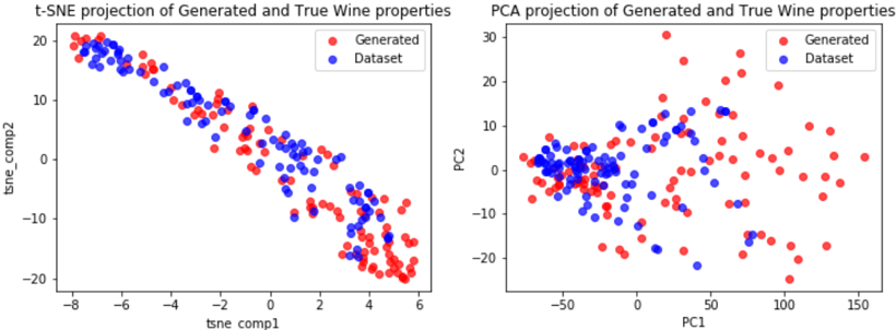
By projecting the generator output as well as the actual training dataset into a lower dimension, using dimensionality reduction techniques such as t-SNE [9Visualizing Data using t-SNEvan der Maaten, L., Hinton, G. · 2008Journal of Machine Learning Research 9, pp. 2579–2605] and Principal Component Analysis (PCA) [10On Lines and Planes of Closest Fit to Systems of Points in SpacePearson, K. · 1901The London, Edinburgh, and Dublin Philosophical Magazine and Journal of Science 2(11), pp. 559–572The origin of principal component analysis.], we can more clearly visualise and confirm that the generator did indeed learn how to reproduce the underlying probability distribution of the wine quality dataset [8Modeling Wine Preferences by Data Mining from Physicochemical PropertiesCortez, P., Cerdeira, A., Almeida, F., Matos, T., Reis, J. · 2009Decision Support Systems 47(4), pp. 547–553]. Figure 4 shows the 2-dimensional projections using t-SNE and PCA.

3.1.3 Imitating handwritten digits using DCGAN

GANs need not be restricted to MLP-based architectures. The models used for the generator and discriminator can be swapped with different architectures depending on the task that is being attempted.

In the following experiment, I investigate a GAN’s ability of generating realistic handwritten digits similar to the 28×28 pixel greyscale images found in the MNIST dataset [11The MNIST Database of Handwritten DigitsLeCun, Y., Cortes, C., Burges, C. J. C. · 2010].

My approach to this problem involves using a Deep Convolutional GAN (DCGAN) model, similar to the one in Radford et al. [7Unsupervised Representation Learning with Deep Convolutional Generative Adversarial NetworksRadford, A., Metz, L., Chintala, S. · 2015ICLRDCGAN.]. In this implementation, the architecture was scaled down and adapted for 28×28×1 images, down from the 64×64×3 of the original paper.

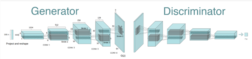
In this experiment, the MLPs in both the generator and discriminator are replaced with Convolutional Neural Networks (CNN).

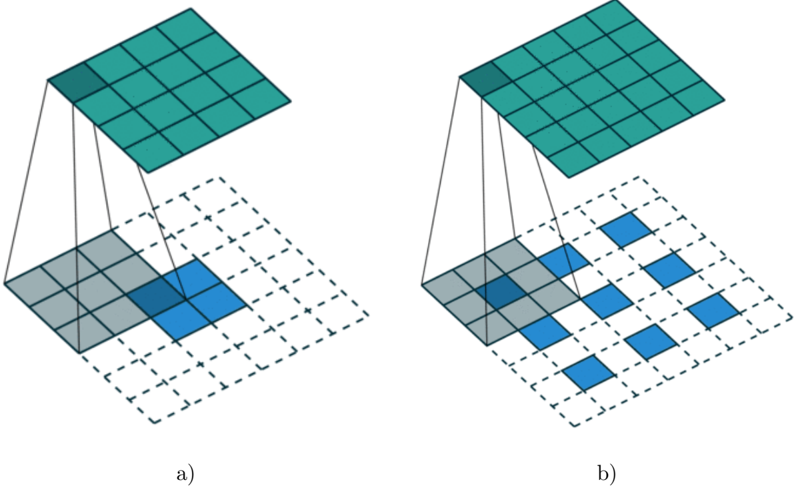
The generator’s architecture is made up of strided transposed convolutional layers (see Figure 29), each of them having their input scaled and shifted using batch normalisation in order to prevent internal covariate shift. As a non-linearity, each layer of the generator uses a ReLU activation, except for the last one which uses a tanh activation in order to squash the output of each pixel between -1 and 1.

Similarly, the discriminator uses strided convolutional layers with a stride of 2, batch normalisation in each of the layers, and a LeakyReLU activation for each of the layers, except for the output, which is squashed using a sigmoid activation.

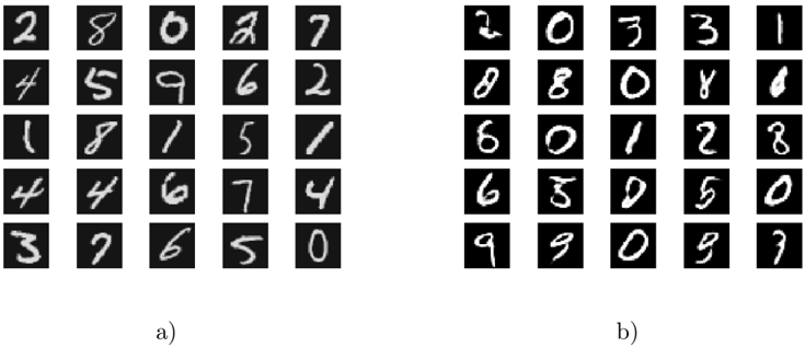
To prevent overfitting in the discriminator, the original DCGAN model had to be altered, introducing dropout at a rate of 0.25 in each of the layers of the discriminator. This modification was successful, and after training we obtained results similar to those of the authors of the original DCGAN paper [7Unsupervised Representation Learning with Deep Convolutional Generative Adversarial NetworksRadford, A., Metz, L., Chintala, S. · 2015ICLRDCGAN.]. These results are shown in Figure 6.

3.2 AnoGAN: GAN-based Outlier Detection Model

Building on the outlier detection techniques described in Chapter 2, and the description of the GAN framework from Section 2.2, I introduce AnoGAN: an outlier detection model that uses a Generative Adversarial Network in order to identify and highlight anomalous regions in medical imaging files [12Unsupervised Anomaly Detection with Generative Adversarial Networks to Guide Marker DiscoverySchlegl, T., Seeböck, P., Waldstein, S. M., Schmidt-Erfurth, U., Langs, G. · 2017Information Processing in Medical Imaging (IPMI)The AnoGAN paper this project builds on.].

In this chapter, I detail the structure of the AnoGAN model, as well as how it can be applied to medical imaging data in order to flag anomalous samples and highlight anomalous regions.

I will then present my own AnoGAN implementation, adapted for outlier detection in the MNIST dataset.

Finally, I will also tackle some of the shortcomings of the AnoGAN framework towards the end of this chapter.

In Schlegl et al. [12Unsupervised Anomaly Detection with Generative Adversarial Networks to Guide Marker DiscoverySchlegl, T., Seeböck, P., Waldstein, S. M., Schmidt-Erfurth, U., Langs, G. · 2017Information Processing in Medical Imaging (IPMI)The AnoGAN paper this project builds on.], the authors propose an unsupervised method of learning a generative representation of local anatomical features, where GANs are trained to learn a generative model of features that make up healthy anatomical images.

After this model is trained on healthy data, the degree of ‘outlyingness’ of a test candidate is determined from the reconstruction error between the most similar image generated by the trained generator, and the test candidate.

Anomalous images are identified by having a high reconstruction error when compared to a generated sample. Theoretically, as a GAN is only learning the latent space representation of ‘healthy’ data, an anomalous test candidate would be impossible for the generator to imitate, and so its latent space mapping would fall outside the learned manifold of the generator after training.

Looking back at the Outlier Detection literature reviewed in Chapter 2, we can classify AnoGAN as a mix between a probabilistic and a reconstruction-based outlier detection model. The probabilistic nature of this model comes from the GAN component learning the underlying distribution of ’normality’, while the reconstruction side is brought forward by the backpropagation algorithm, which attempts to minimise a reconstruction error between the test candidate and the generated output.

The model implemented by the authors uses the DCGAN model proposed by Radford et al. [7Unsupervised Representation Learning with Deep Convolutional Generative Adversarial NetworksRadford, A., Metz, L., Chintala, S. · 2015ICLRDCGAN.]. Instead of using an MLP to map the noise vector to the output, the authors make use of strided transposed convolutional and convolutional layers in the generator and discriminator. The architecture of AnoGAN is presented in Figure 7.

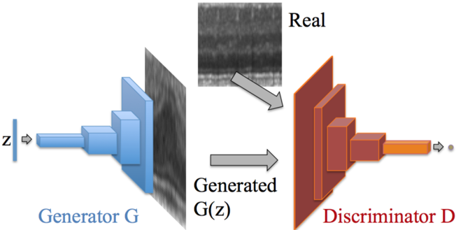
In AnoGAN, the generator is used as a function that can construct healthy anatomical images from random noise vectors $z$. When investigating a test candidate for outlier detection, we aim to find a variable $z$ in the latent space of the generator that, when mapped through the generator function $G(z)$, will yield an image that is visually similar to the test candidate.

The main issue with GANs, however, comes from having the generator map random noise vectors to meaningful output. As such, we do not have a direct mapping between a generated image and a point lying on the latent space of the generator. This mapping is thus inferred through the use of computer vision algorithms.

In order to find a latent space mapping of the test image, we sample $z$ randomly, and then progressively update its values through $1, 2, \ldots, \Gamma$ backpropagation steps, minimising a loss function between the generated image and the test image.

In the original paper, the authors define an anomaly loss for updating the latent variable $z$, which is comprised of two separate loss functions: the residual loss $\mathcal{L}_R(z_\gamma \mid \mathbf{x})$ and the discriminator loss $\mathcal{L}_D(z_\gamma \mid \mathbf{x})$, both conditioned on the input $\mathbf{x}$.

The residual loss function computes the sum of the pointwise difference between the input image and the image generated by the generator from z :

where $z_\gamma$ is the random input vector $z$ at backpropagation step $\gamma \in \{1, 2, \ldots, \Gamma\}$.

The discriminator loss makes use of the trained discriminator to compute a dissimilarity measure between the test and generated images.

Instead of using the discriminator to classify between real/fake input, the last fully-connected layer of the discriminator is removed, effectively using the penultimate fully-connected layer, as well as all the previous convolutional layers for computing a loss. Since the convolutional layers learn to extract patterns from images, we are essentially using our modified discriminator as a feature extractor rather than a ‘real’/‘fake’ classifier.

Thus, the discrimination loss is computed as:

where $f(\cdot)$ is the penultimate fully-connected layer of the discriminator.

The final loss function will be the weighted sum of these two losses:

with $\lambda$ balancing how much each of the individual losses contributes to the anomaly score.

The anomaly score of the input image is computed using the input vector $z_\Gamma$, after $\Gamma$ backpropagation steps, and is given in Equation 7.

where $R(\mathbf{x}) = \mathcal{L}_R(z_\Gamma \mid \mathbf{x})$ and $D(\mathbf{x}) = \mathcal{L}_D(z_\Gamma \mid \mathbf{x})$.

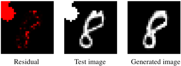
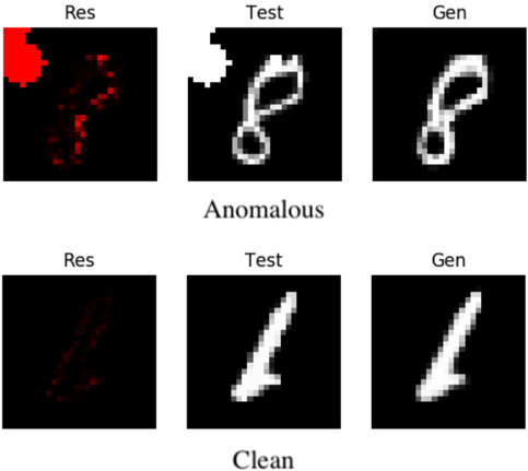
Anomalous regions in images can be pinpointed and highlighted by computing a residual image between the test candidate and the generated image at backpropagation step $\Gamma$. This residual image is given in Equation 8.

3.2.1 AnoGAN: Adaptation for MNIST

By building on the work of Schlegl et al. [12Unsupervised Anomaly Detection with Generative Adversarial Networks to Guide Marker DiscoverySchlegl, T., Seeböck, P., Waldstein, S. M., Schmidt-Erfurth, U., Langs, G. · 2017Information Processing in Medical Imaging (IPMI)The AnoGAN paper this project builds on.], I adapted and implemented a version of AnoGAN that is capable of identifying anomalous handwritten digit images, as well as highlighting the anomalous regions.

For this implementation, I based my model on the DCGAN model used for MNIST digit generation in Section 3.1.3, only adding the backpropagation outlier detection algorithm to this model.

After training, the generator is replicated for image generation. During the anomaly detection process, the generator’s weights are kept frozen, and the only variable that is updated through backpropagation is $z$ itself, by minimising the anomaly score of Equation 7.

Given an image test set $\mathbf{X}_t = \{X_t^{(1)}, X_t^{(2)}, \ldots, X_t^{(m)}\}$, the anomaly score after $\Gamma$ backpropagation steps is extracted using the outlier detection backpropagation algorithm, yielding scores $\{A(X_t^{(1)}), A(X_t^{(2)}), \ldots, A(X_t^{(m)})\}$.

3.2.1.1 Results

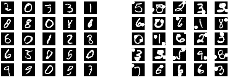
The MNIST AnoGAN test set contains 150 MNIST digits sampled from the MNIST test set. Out of these, 100 instances are clean images, while 50 of them are images which had blobs of random sizes added at random positions throughout the image (see Figure 9).

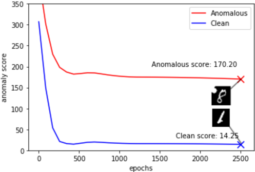
After running the anomaly detection algorithm, the convergence anomaly score $A(X_t^{(i)})$ of each test image can be used for clean/anomalous classification. This can be done dynamically, without requiring us to impose a hard threshold value on the anomaly score of a test image. The significant difference in the convergence values of anomaly scores between clean and anomalous images offers a wide enough margin for classification, as can be seen in Figure 10.

This clear separation between losses is also seen in the residual images, where anomalous images have much larger anomalous areas (see Figure 11).

For clean/anomalous classification based on anomaly score, I used a Gaussian Mixture Model (GMM), a generative model in which random variables are sampled from a mixture of a finite number of Gaussian probability distributions. This can be thought of as a soft version of the k-means algorithm, where instead of performing a hard assignment on a data point to belong to an arbitrary cluster, we assign probabilities of a data point belonging to each of the clusters.

A problem that usually comes up when using a Gaussian Mixture Model is that the data is usually unlabelled, and therefore an educated guess has to be made as to how many classes (clusters) the model should use. In this case, this is not a problem, since we know that we want to classify the data as either clean or anomalous, so we will have only two clusters.

In order to compute the clusters, GMM uses the Estimation-Maximisation (EM) algorithm, which computes the likelihood of each data point with respect to a cluster, and then updates the cluster’s prototype to maximise the likelihood of the data being generated from that cluster’s distribution. Figure 12 shows a GMM fitted to a scatter plot of residual losses against discriminator losses for the 150 test images.

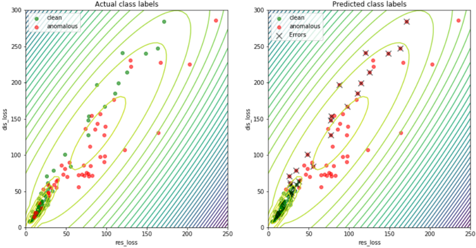
I fitted two GMMs to the anomaly detection results on the 150 test images. One of them is a 2D GMM fitted around the residual-discriminator loss scatter plot, the other being fitted on the anomaly scores of the test images. Benchmarking these two models using a confusion matrix (see Table 4), the anomaly score can be observed to be a more accurate metric for outlier detection, as opposed to the residual or discriminator losses by themselves.

Table 4. Confusion matrix metrics for the fitted Gaussian Mixture Models. The 2D GMM was fitted on the residual loss against the discriminator loss; the 1D GMM was fitted on the anomaly score of the images.

From Figure 12, it can be observed that the clean images tend to cluster together in regions of low loss values, while the anomalous images are scattered further apart from each other in regions of higher loss values.

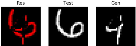
This is normal and expected, as during the adversarial training process, the AnoGAN learns the criteria for normalcy in clean images. Therefore, all clean images will have to meet the same criteria, and thus clustering tightly together in a region of small loss values. On the other hand, each anomalous image can be anomalous in its unique way, and therefore it is to be expected for the cluster of anomalous images to have a higher variance in loss values.

3.2.1.2 Interpolation errors

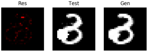
An interesting pattern arises when clean images have high loss values, as could be observed in Figure 12. This clearly should not be the case, as the AnoGAN model has seen very similar images in the training stage. Both Figure 13 and Figure 14 show how the generator mistakenly generates digits that it has never seen during training, and which do not look anything like the digits used in the training stage. In Figure 13, it appears that the generator is trying to generate the digit 4, when it should clearly be aiming to generate the digit 6.

Similarly, all anomalous images should have higher loss values than the clean images, as the model hasn’t seen anything like them during the training process. This is clearly not the case in Figure 14, where the generator might be interpreting the test image as a backwards digit 6. This is clearly in error, and should not happen during the anomaly detection process.

We hypothesize that this might be due to a separated latent space from which the random noise vector $z$ is being sampled.

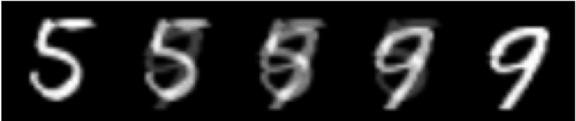
By having gaps between classes, the noise vector $z$ can fall into a region between the classes, forcing the generator to interpolate between them and generate mangled digits. Figure 15 shows latent space interpolation between two digits.

3.3 Generalising the AnoGAN model

3.3.1 Finding a substitute residual loss

For testing the applicability of the AnoGAN model to datasets outside the realm of Medical Imaging and Computer Vision, the AnoGAN model was benchmarked against the Wine Quality dataset [8Modeling Wine Preferences by Data Mining from Physicochemical PropertiesCortez, P., Cerdeira, A., Almeida, F., Matos, T., Reis, J. · 2009Decision Support Systems 47(4), pp. 547–553] described in Section 3.1.2.

The model used for this benchmark was almost identical to the model used for MNIST outlier detection in Section 3.2.1, the only modification being altering the shape of the generator’s output from a 784-dimensional to an 11-dimensional vector, and adapting the discriminator’s expected input shape to account for this. This was done to accommodate the Wine Quality dataset, which consists of 11-dimensional vectors.

The AnoGAN experiment was re-run on the Wine Quality dataset, training the GAN component for 30,000 epochs, while using only ‘clean’ (normal wines, excluding wines with quality 9 and above) as training data.

After performing outlier detection on a test set consisting of 700 wines, out of which 35 (5%) of them had quality 9 or above, a high degree of overlap can be noticed in the loss values between outliers and normal data (Figure 16).

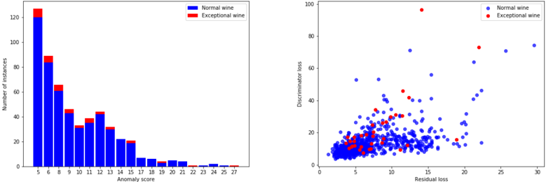
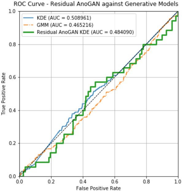
In benchmarks, the standard AnoGAN with residual loss obtains a performance which is no better than the performance of other outlier detection models such as the Gaussian Mixture Model or Kernel Density Estimation (Figure 17).

The main advantage of using a GAN for outlier detection was the possibility of creating a separation between clean and anomalous data, mainly represented through the discrepancy in loss values. As can be seen from Figure 16, this boundary cannot be extracted from this result of anomaly detection.

This problem was not encountered while running the AnoGAN experiment on the MNIST dataset, even though the only variables between the two experiments were the datasets and the output shape of the generator. This difference may be brought forward by the increased sparsity of the 784-dimensional MNIST dataset, where the background of each digit (value 0) constitutes the bulk of the feature-vector. Because of the denser feature vectors exhibited in the wine quality dataset, it might be harder for the backpropagation algorithm to converge on a correct latent space representation of the test candidate.

This problem could be avoided by evaluating a distribution of test candidates against the outlier detection algorithm, and using a similarity metric between the distribution of the test candidate and the distribution of the generated output of the generator.

Since the generator is only capable of generating data that follows the same distribution as the one that was seen during training, any items outside the distribution of the generator can be flagged as anomalous, thus replacing the residual loss described in Schlegl et al. [12Unsupervised Anomaly Detection with Generative Adversarial Networks to Guide Marker DiscoverySchlegl, T., Seeböck, P., Waldstein, S. M., Schmidt-Erfurth, U., Langs, G. · 2017Information Processing in Medical Imaging (IPMI)The AnoGAN paper this project builds on.].

I hypothesise that evaluating a measure of similarity between a sample of test candidates and a sample from the trained generator will provide a performance increase for the AnoGAN outlier detection algorithm.

3.3.2 Estimating the data distribution

In order to compute the information about the underlying distribution of each of the samples, each of the samples is estimated using Kernel Density Estimation (KDE).

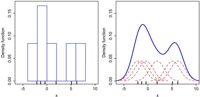
KDE is a technique that is similar to histogram binning, which replaces the need to parameterise bin numbers and bin edges, by placing a kernel function on top of each point in the sample (see Figure 18). The probability distribution of the estimation is thus computed from the contributions of each of the kernels.

For the purpose of this project, the AnoGAN model was implemented in the TensorFlow [15TensorFlow: Large-Scale Machine Learning on Heterogeneous Distributed SystemsAbadi, M., Agarwal, A., Barham, P., et al. · 2016] Python library. As TensorFlow does not include functionality for KDE, I implemented my own library of KDE functions from scratch (see Appendix B).

3.3.3 Bhattacharyya distance as similarity measure

While the Kullback–Leibler divergence (Equation 10) can be used as a similarity metric between two distributions by investigating the information content of each, KL-divergence is not a valid distance metric, due to its lack of symmetry $\left( \mathrm{KL}(p \parallel q) \neq \mathrm{KL}(q \parallel p) \right)$.

The Bhattacharyya distance [16On a Measure of Divergence between Two Multinomial PopulationsBhattacharyya, A. · 1946Sankhyā: The Indian Journal of Statistics 7(4), pp. 401–406], however, is a valid statistical distance: it is symmetric, and so can be used to evaluate the similarity of two distributions.

The probability distributions $p$ and $q$ are estimated using the aforementioned Kernel Density Estimation technique (using the custom TensorFlow libraries mentioned above), and thus, the residual loss is substituted for the Bhattacharyya distance in the anomaly detection algorithm.

Chapter 4 - Evaluation

By evaluating the distribution of the test candidate against the distribution of generated data, and using Bhattacharyya distance as a similarity metric, I hypothesise that this extended AnoGAN form is capable of outperforming other generative outlier detection models, as well as outperforming the classic, residual-loss-based AnoGAN described by Schlegl et al. [12Unsupervised Anomaly Detection with Generative Adversarial Networks to Guide Marker DiscoverySchlegl, T., Seeböck, P., Waldstein, S. M., Schmidt-Erfurth, U., Langs, G. · 2017Information Processing in Medical Imaging (IPMI)The AnoGAN paper this project builds on.].

The performance of the extended AnoGAN is benchmarked against some of the generative outlier detection systems presented in Chapter 2. The focus falls specifically on generative (or probabilistic) models, in order to evaluate whether the adversarial component of generative learning in GANs brings a benefit.

4.1 Test dataset

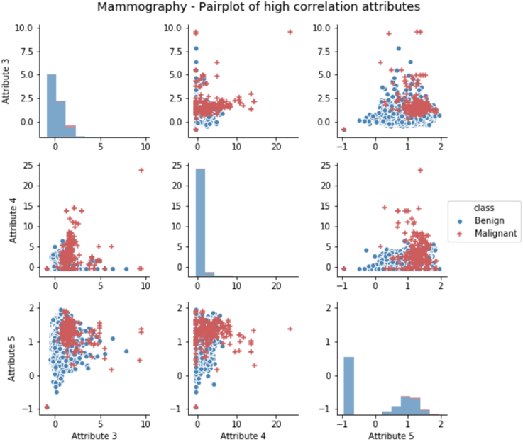
All the models that are evaluated in this section are going to be tested against the mammography dataset from Woods et al. [17Comparative Evaluation of Pattern Recognition Techniques for Detection of Microcalcifications in MammographyWoods, K. S., Doss, C. C., Bowyer, K. W., Solka, J. L., Priebe, C. E., Kegelmeyer Jr., W. P. · 1993International Journal of Pattern Recognition and Artificial Intelligence 7(6), pp. 1417–1436Source of the mammography benchmark dataset.], which is made up of 11,183 samples of various features detected during mammographies. Out of the 11,183 samples, 260 are samples in which a malignancy has been detected. The small number of samples which are malignant makes this dataset very useful for testing outlier detection models.

Even though the model does not have names for the attributes, these are not needed for inferring properties of the dataset for data mining / data analysis work.

Table 5. Top two entries in the mammography dataset.

4.2 AnoGAN benchmark against generative models

AnoGAN is compared against two generative models for outlier detection, namely the Gaussian Mixture Model (GMM), a parametric model, and Kernel Density Estimation (KDE), a non-parametric model. Also, the extended Bhattacharyya AnoGAN is benchmarked against the original, residual-loss AnoGAN described in Schlegl et al. [12Unsupervised Anomaly Detection with Generative Adversarial Networks to Guide Marker DiscoverySchlegl, T., Seeböck, P., Waldstein, S. M., Schmidt-Erfurth, U., Langs, G. · 2017Information Processing in Medical Imaging (IPMI)The AnoGAN paper this project builds on.] (adapted to this dataset).

In KDE, the distribution of the data is estimated by placing kernel functions on each of the points, and then computing the contribution of each kernel to the probability density. Based on the prior assumption about the number of outliers to be expected in the dataset, $n$, the $n$ lowest-likelihood members of the distribution are being flagged as outliers.

In GMM, a mixture made up of a finite number of Gaussian distributions is being fit on the data. During evaluation, similar to the KDE case, a threshold is being imposed on the data. If the test candidate has a value below the threshold with respect to each of the Gaussian clusters, it is flagged as being an outlier.

In this implementation, the number of Gaussian clusters to consider is being parameterised.

For AnoGAN, the test dataset is grouped together in samples of 30 mammogram readings. The test groups were split between groups consisting of 100% clean data, and groups containing 100% anomalous data.

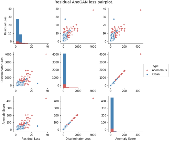
After anomaly training, the Bhattacharyya, discriminator and anomaly loss at convergence is being collected from each of the groups. A plot of these loss values can be seen in Figure 20.

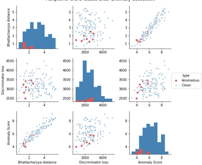
The bizarre observation that can be made in this situation is that the losses of anomalous samples have lower values than losses of clean samples. This is contrary to what was expected from this experiment.

Nevertheless, one success of this extended form of the AnoGAN outlier detection algorithm was increasing between-class separation.

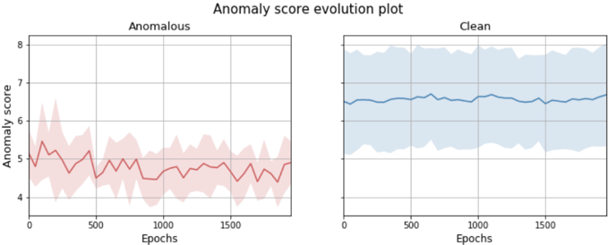
Investigating the evolution of the anomaly score across training for all test candidates, the anomaly score can be seen not to converge to a value much smaller than the initial starting value. Figure 21 shows a time-series plot of the anomaly score across the whole outlier detection process.

Moving forward with this result, a KDE model is fitted on the anomaly score of the test candidates. As the test dataset includes 8 anomalous groups and 130 clean groups, a threshold on the likelihood is imposed at 0.062 $\left( 8/130 \right)$.

Table 6. Benchmark — AnoGAN against generative outlier detection models. Accuracy metrics were computed for AnoGAN by fitting a KDE model onto the anomaly score produced by each test candidate.

Though all four models have very high accuracies, since accuracy is computed as:

the high degree of accuracy of all four models is due to the fact that outliers make up a very small proportion of the dataset (1.43% for test set of KDE/GMM/Residual AnoGAN and 5.97% for Bhattacharyya AnoGAN test set).

However, by looking at the Recall (true positives against actual positives), each model’s performance can be correctly judged.

From the beginning, it is clear that the Residual AnoGAN model outperforms all other models, correctly identifying more than half of the outliers in the dataset.

The performance of Residual AnoGAN can be attributed to the much improved class separation that it achieves by mapping anomalies to a high anomaly score. This can be observed in Figure 22.

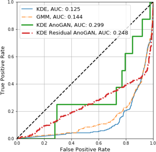
On the other hand, from the receiver operating characteristic curve (Figure 23), the extended AnoGAN model does have a better true-positive to false-positive ratio than all other models, judged by its AUC score.

After running this evaluation, the hypothesis can be safely rejected, justified by the significant discrepancy in Recall values between the extended Bhattacharyya AnoGAN model and the other models that were investigated.

Chapter 5 - Future Work

5.1 Latent space smoothing

Section 3.2.1.2 detailed how the process of outlier detection using GANs can be negatively affected by a non-smooth latent space of the generator.

In the backpropagation algorithm that finds a latent space representation for the test candidate, this can lead to generated images that look similar to anomalous images, thus leading to false negative results during the anomaly detection process.

One way to overcome this issue is to smooth out the latent space of the generator.

While this is not easily possible with a standard GAN, because the generator uses random noise as input, other techniques might be able to help with the smoothing of the latent space.

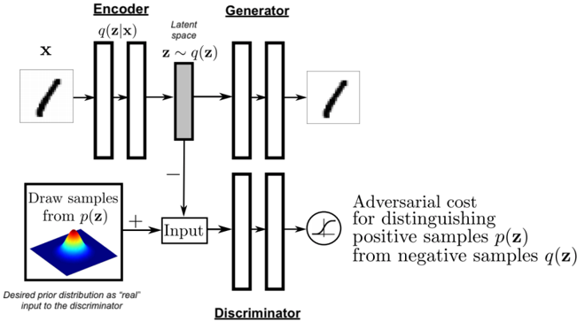
One such technique, detailed in Makhzani et al. [18Adversarial AutoencodersMakhzani, A., Shlens, J., Jaitly, N., Goodfellow, I., Frey, B. · 2015], uses a generator-discriminator adversarial pair in conjunction with an autoencoder to impose a prior distribution on the latent space of the model (Figure 24).

5.2 Fully-unsupervised anomaly detection

Finding anomalies using AnoGAN involves applying a generative model on the losses of the test candidate, and thresholding the lowest likelihood candidates by using a prior probability of outliers existing in the dataset.

An interesting extension to this model could come from unsupervised GAN training using training data that contains a small proportion of outliers. In some experiments, I have found that adding a small amount of outlier images to the training of a GAN on MNIST did not affect the output of the generator adversely.

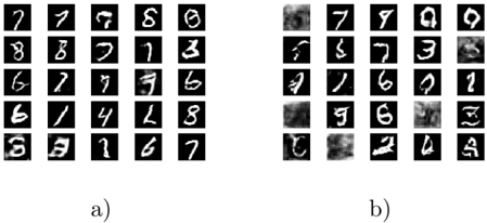
This could mean that the generator learns to map the most important features of the training data distribution. If this is the case, the AnoGAN model described in this project could still be used for identifying outliers without the need of training a GAN on strictly outlier-free data.

Chapter 6 - Conclusion

The work carried out in this project has investigated the use of Generative Adversarial Networks for training generative models to learn complex data distributions in an adversarial context, as well as representing complex high-dimensional data in a lower dimensional latent space embedding.

By exploiting a GAN’s ability to generate data from a latent space, this project has shown how the absence of a latent space embedding for a test candidate can be interpreted as the presence of an outlier.

Despite promising results on Computer Vision and Medical Imaging tasks, further work needs to be carried out to create an accurate, generic and robust GAN-based outlier detection model.

Chapter 7 - Project Management

I prioritised my time between modules, assignments and other commitments such that I could dedicate approximately half of the total study time in this academic year towards the Individual Project.

Starting from the beginning of the year, I treated this project as a typical software engineering project with requirements and deliverables, and as such I planned my work using some ScrumWhat is Scrum? methodologies:

• All tasks were kept in a backlog, using Asanaasana.com , and were labelled based on their importance, urgency and type.
• At the end of each week, all tasks in the backlog were reviewed in a ‘Sprint Planning’ session, and their priority and urgency changed to best reflect their current status. Any new tasks that had to be done were added, while removing tasks that have been descoped from the project.
• At the beginning of each week, a new Sprint Board for the current week would be created, with a deliverable goal. All relevant tasks were added, keeping in mind the time commitment needed for each task, and the time available for the current week.
• At the beginning of each day, a small selection of tasks were selected to be completed during that day.
• Any items that were blocked due to outside influences were labelled ‘BLOCKED’ and placed back into the week’s backlog.

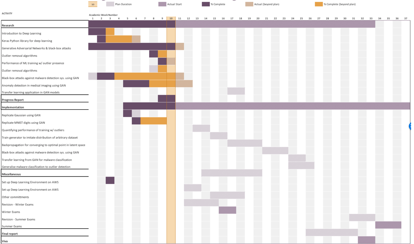
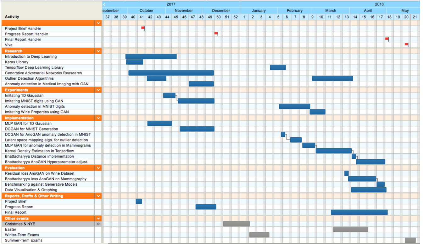
Following a Scrum methodology resulted in many tasks appearing in parallel in the Gantt Chart. This was due to the weekly and daily reallocation of priorities and also blocked tasks.

Appendix

Appendix A — Model hyperparameters

1-dimensional Gaussian experiment

Both networks are multilayer perceptrons with one hidden layer, optimised with Adam at a learning rate of 0.0002.

Wine quality experiment

Optimised with Adam at a learning rate of 0.0002 and a beta1 value of 0.9. Dropout at a rate of 0.5 was added to all layers of both the discriminator and the generator.

Appendix B

TensorFlow implementations

TODO

Appendix C

Convolutional arithmetic

Appendix D

Dataset description

D.1 Wine quality dataset

The wine quality dataset presented in Cortez et al. [8Modeling Wine Preferences by Data Mining from Physicochemical PropertiesCortez, P., Cerdeira, A., Almeida, F., Matos, T., Reis, J. · 2009Decision Support Systems 47(4), pp. 547–553] is made up of red and white wines from the Portuguese ‘Vinho Verde’ collection. It is made up of 1599 red and 4898 white wine instances.

Table 7. Input variables (based on physicochemical tests).

Table 8. Output variable (based on sensory data).

D.2 MNIST: Handwritten digit dataset